
Introduction
The PID Controller is a Proportional – Integral – Derivative controller or three-term controller. It is a control loop mechanism that uses feedback and is widely used in industrial control systems and in a variety of other applications that require constantly configured control. A PID controller continuously calculates an error value e (t) as the difference between a desired setpoint (SetPoint -SP) and the current value of a measurable process variable (Process Variable PV) and applies a correction based on analog, integral and derivative term (denoted by P, I and D respectively), hence the name.
In practice, it automatically applies an accurate and responsive correction to a control function. An everyday example is cruise control in a car, where climbing a hill would reduce speed if there was only constant engine power. The controller PID algorithm restores the measured speed to the desired speed with minimal delay and exceedance by increasing the motor output power in a controlled manner.
Controller operation
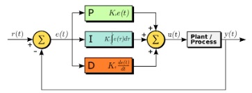
The feature of the PID controller is the ability to use the three control terms of analog, integral and derivative influence on the controller output to implement accurate and optimal control. The controller block diagram shown below shows the principles of how these terms are created and applied. Displays a PID controller, which continuously calculates an error value e (t) as the difference between a desired setpoint SP = r (t) and a measured process variable PV = y (t) e (t) = r (t) -y (t) and applies a correction based on a proportional, integral and derivative term. The controller tries to minimize the error over time by adjusting a control variable u (t), such as e.g. opening a control valve,to a new value determined by a weighted sum of the control conditions.
How does the PID controller work?
The overall output of the PID controller is a combination of the three terms as shown in the figure above, P, I and D
The term P is proportional to the current value of the error SP−PV = e(t).
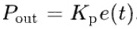
For example, if the error is large and positive, the control output will be proportionally large and positive, taking into account the gain factor Kp. Only P control (Proportional) is sufficient and a system works well when:
a. The system is simple and responds quickly.
b. Absolute accuracy in the final result is not required.
c. It is acceptable to have a little error in the steady-state (final state).
d. You have no problem with a constant deviation from the setpoint.
Thus, when only P control operates in a system, there are limitations:
- Steady-state error:
a. P control cannot completely eliminate the error.
b. As you approach the desired value, the error decreases → so the correction also decreases → and stops before you reach the setpoint. - Power limitation:
a. If you make the proportional coefficient Kp too large, to “push” it harder, then:
a1. The system becomes unstable.
a2. You may have oscillations or overshoot. - Bad behavior in slow or complex systems:
a. In systems with inertia (such as thermal or mechanical), P control alone does not have time or is slow to react correctly.
For example, let’s say you’re controlling a motor to reach a specific speed.
With P alone, it can get close to the target, but:
a. It may stop at 98% of the target and never go exactly to 100%.
b. If you increase Kp, it may oscillate around 100% (overshoot → undershoot → overshoot…).
Term I takes into account the previous values of the SP − PV error
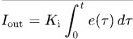
and integrates them over time to produce the term I. For example, if there is a residual error SP − PV after the analog control is applied, the term integral seeks to eliminate the residual error by adding a control result, weight K i , due to the historical cumulative value of the error. When the error is eliminated, the term will stop growing. This will result in a reduction in the analog result as the error decreases, but this is offset by the increasing overall effect.
Term D is the best estimate of the future trend of the SP − PV error,
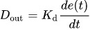
ased on its current rate of change. It is sometimes referred to as “prudential control”, as it essentially seeks to reduce the effect of the SP − PV error by exerting a control influence created by the rate of change of the error. The faster the change, the greater the effect of control or damping. The role of the constant K d in the calculation of the correction D is important.
Application of PID controller in Code
To implement a PID controller in code or an Arduino program, five parameters must be known:
- proportional constant K p
- integral constant K i
- and derivative constant K d
- entry price (PV)
- and set point value (SP)
The PID calculation must be inside a loop function. The first part of the function should be to determine the time elapsed.
In Arduino, the current time can be determined with the millis () function and the elapsed time is simply:
currentTime = millis ();
elapsedTime = currentTime – previousTime;
Next, the error must be identified:
error = setPoint – input;
Programming on an Arduino simplifies the calculations a lot by using the PID_v1 library. In the example I give you I used the PID_v1 library.
In any case it is necessary to determine the three constants P, I, D. This determination is usually done experimentally and is a laborious process.
Construction
This construction is a continuation of the previous one I did with the two servo motors. In this construction I have added the MPU-9250 sensor which will “drive” the servo motors. See more here.
The most important thing for the construction is the software that we will write so that the movement of the servo motors is now controlled by the sensor and is done smoothly, without oscillations and brings the system to the desired (horizontal) position.
The code of the construction for Arduino UNO is shown below and can be downloaded from here.
/********************************************************
* Author : Manolis Aristovoulidis
* Το πρόγραμμα αυτό χρησιμοποιεί έναν αισθητήρα κίνησης MPU-9250,
* δύο σερβοκινητήρες και έλεγχο PID στην κίνηση των σερβοκινητήρων.
* Με τη λειτουργία του προγράμματος οισερβοκινητήρες κρατουν πάντα σε
* οριζόντια θέση τον αισθητήρα όπως και να περιστρέψουμε τη βάση της κατασκευής
*
* This program uses an MPU-9250 motion sensor,
* two servomotors and PID control in servomotors.
* With the operation of the program, motors always keep on
* position the sensor horizontally as well as rotate the base of the construction
* Date : 27/11/2021
*
 ********************************************************/
#include <Wire.h>
#include <MPU9250.h>
#include <Servo.h>
#include <PID_v1.h>

Servo servo_x;      // δημιουργία ενός servo object για τον έλεγχο του servo
Servo servo_y;      // creating a servo object to control the servo

int val_x = 100;     // Αρχική γωνια για το servo_x    Home corner for servo_x
int val_y = 100;    // Αρχική γωνια για το servo_y    Home corner for servo_y

 // an MPU9250 object with the MPU-9250 sensor on I2C bus 0 with address 0x68
 MPU9250 IMU(Wire,0x68);

int status;

 //Acc Variables

float rad_to_deg = 180/3.141592654;           //Αυτή η τιμή είναι για τη μετατροπή ακτινίων σε μοίρες
float Acc_rawX, Acc_rawY, Acc_rawZ;           //Εδώ αποθηκεύουμε ανεπεξέργαστα δεδομένα από το επιταχυνσιόμετρο
float Acc_angle_x, Acc_angle_y;               //Εδώ αποθηκεύουμε τις τιμές γωνίας που υπολογίσαμε για το επιταχυνσιόμετρο
float SUp_Acc_angle_x, SUp_Acc_angle_y;        //SetUp angles
float Gyr_rawX, Gyr_rawY, Gyr_rawZ;           //Εδώ αποθηκεύουμε ανεπεξέργαστα δεδομένα από το γυροσκόπιο
float Gyro_angle_x, Gyro_angle_y;             //Εδώ αποθηκεύουμε τις τιμές γωνίας που υπολογίσαμε για το γυροσκόπιο

float Total_angle_x, Total_angle_y;           //Εδώ αποθηκεύουμε τις τελικες ολικές γωνίες
float elapsedTime, timeNow, timePrev;         //Μεταβλητές για τον έλεγχο χρόνου


//Καθορίζουμε τις μεταβλητές που θα συνδεθούν με τα αντικείμενα PID_x και PID_y
double Setpoint_x, Input_x, Output_x;
double Setpoint_y, Input_y, Output_y;

//Καθορίζουμε τις αρχικές παραμέτρους συντονισμού
double x_Kp=2.0, x_Ki=0.5, x_Kd=0.01;
double y_Kp=2.0, y_Ki=0.5, y_Kd=0.01;

//Δημιουργούμε τα αντικείμενα PID
PID PID_x(&Input_x, &Output_x, &Setpoint_x, x_Kp, x_Ki, x_Kd, DIRECT);
PID PID_y(&Input_y, &Output_y, &Setpoint_y, y_Kp, y_Ki, y_Kd, DIRECT);

void setup()
{
  Serial.begin(115200);
  while(!Serial) {}

    servo_x.attach(4);    //κάνει προσάρτηση του servo στο pin 4 του servo object // attachs the servo to pin 4 of   the servo object
    servo_y.attach(5);    //κάνει προσάρτηση του servo στο pin 5 του servo object // attachs the servo to pin 5 of the servo object

    //περιστοφή των σερβοκινητήρων
    servo_x.write(val_x);   //Μετά από πειραματισμούς αυτή είναι η      //After experimentation this is
    servo_y.write(val_y);   //οριζόντια θέση για τη βάση του MPU9250    // horizontal position for the MPU9250 base

    delay(1000);

    // start communication with IMU
    status = IMU.begin();
    if (status < 0) {
      Serial.println("IMU initialization unsuccessful");
      Serial.println("Check IMU wiring or try cycling power");
      Serial.print("Status: ");
      Serial.println(status);
      while(1) {}
    }
  /* Default values of MPU9250
   * accel range to 16G as default
   * gyro range to 2000DPS as default
   * bandwidth to 184Hz as default
   * sample rate divider to 0 as default
   *
   */
   delay(3000);

    IMU.readSensor();
    Acc_rawX = IMU.getAccelX_mss();
    Acc_rawY = IMU.getAccelY_mss();
    Acc_rawZ = IMU.getAccelZ_mss();


    /*---Y---*/
    SUp_Acc_angle_x = (atan((Acc_rawY)/sqrt(pow((Acc_rawX),2) + pow((Acc_rawZ),2)))*rad_to_deg) ;
    /*---Y---*/
    SUp_Acc_angle_y = (atan(-1*(Acc_rawX)/sqrt(pow((Acc_rawY),2) + pow((Acc_rawZ),2)))*rad_to_deg) ;

  //Input_x = 0.0;
  Input_x = SUp_Acc_angle_x;
  Setpoint_x = SUp_Acc_angle_x;
  //Setpoint_x = 0.0;

  //Input_y = 0.0;
  //Setpoint_y = 0.0;
  Input_y = SUp_Acc_angle_y;
  Setpoint_y = SUp_Acc_angle_y;

  double mini = -90;
  double maxi = 90;
  PID_x.SetOutputLimits(mini, maxi);  //ορίζουμε τα όρια ελάχιστης - μέγιστης τιμής που
  PID_y.SetOutputLimits(mini, maxi);  //θα μας επιστρέφει ο μηχανισμός ελέγχου PID
  //turn the PID on
  PID_x.SetMode(AUTOMATIC);
  PID_y.SetMode(AUTOMATIC);
}

void loop()
{
  timePrev = timeNow;  // η προηγούμενη ώρα αποθηκεύεται πριν διαβάσουμε την πραγματική ώρα
  timeNow = millis();  // Ανάγνωση πραγματικής ώρας
  elapsedTime = (timeNow - timePrev) / 1000;

  IMU.readSensor();
  Acc_rawX = IMU.getAccelX_mss();
  Acc_rawY = IMU.getAccelY_mss();
  Acc_rawZ = IMU.getAccelZ_mss();

  Gyr_rawX=IMU.getGyroX_rads();
  Gyr_rawY=IMU.getGyroY_rads();

  /*---Y---*/
  Acc_angle_x = (atan((Acc_rawY)/sqrt(pow((Acc_rawX),2) + pow((Acc_rawZ),2)))*rad_to_deg) ;
  /*---Y---*/
  Acc_angle_y = (atan(-1*(Acc_rawX)/sqrt(pow((Acc_rawY),2) + pow((Acc_rawZ),2)))*rad_to_deg) ;

  Gyro_angle_x = Gyr_rawX*elapsedTime;
  /*---X---*/
  Gyro_angle_y = Gyr_rawY*elapsedTime;


  Total_angle_x = 0.98 *(Total_angle_x + Gyro_angle_x) + 0.02*Acc_angle_x;
  Total_angle_y = 0.98 *(Total_angle_y + Gyro_angle_y) + 0.02*Acc_angle_y;

  Input_x = Total_angle_x;
  Input_y = Total_angle_y;

  PID_x.Compute();
  PID_y.Compute();

  servo_x.write(Output_x + val_x );        // ρυθμίζει τη θέση του servo στην τιμή της κλίμακας
  servo_y.write(val_y - Output_y);
  //Serial.print(Input_x);                   // εκτυπώσεις για την παρακολούθηση του μηχανισμού σε λειτουργία
  //Serial.print(",");
  //Serial.println(Input_y);
  delay(40);
}